SynthPix: A lightspeed PIV images generator 🌊

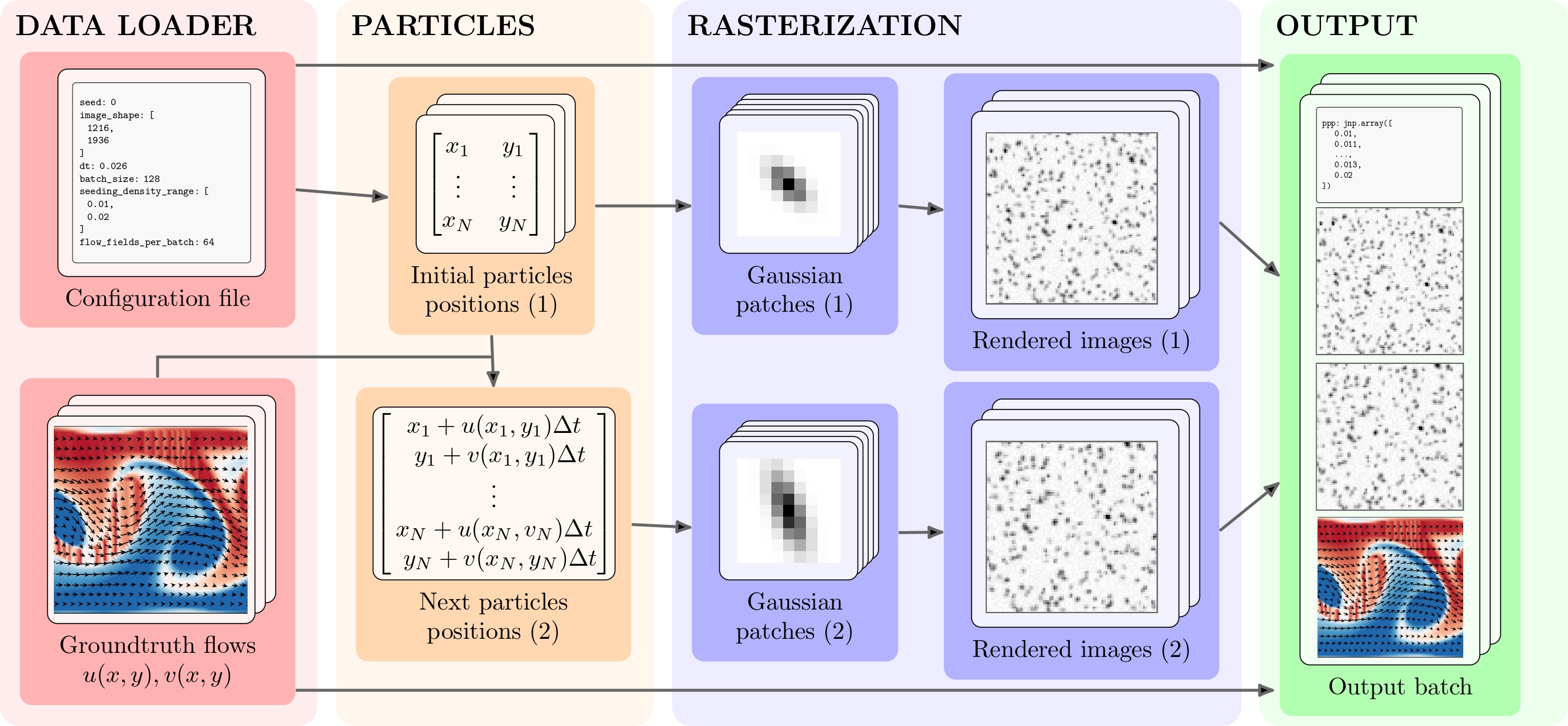
SynthPix is a synthetic image generator for Particle Image Velocimetry (PIV) with a focus on performance and parallelism on accelerators, implemented in JAX. SynthPix supports the same configuration parameters as existing tools but achieves a throughput several orders of magnitude higher in image-pair generation per second, enabling comprehensive validation and comparison of PIV algorithms, rapid experimental design iterations, and the development of data-hungry methods.

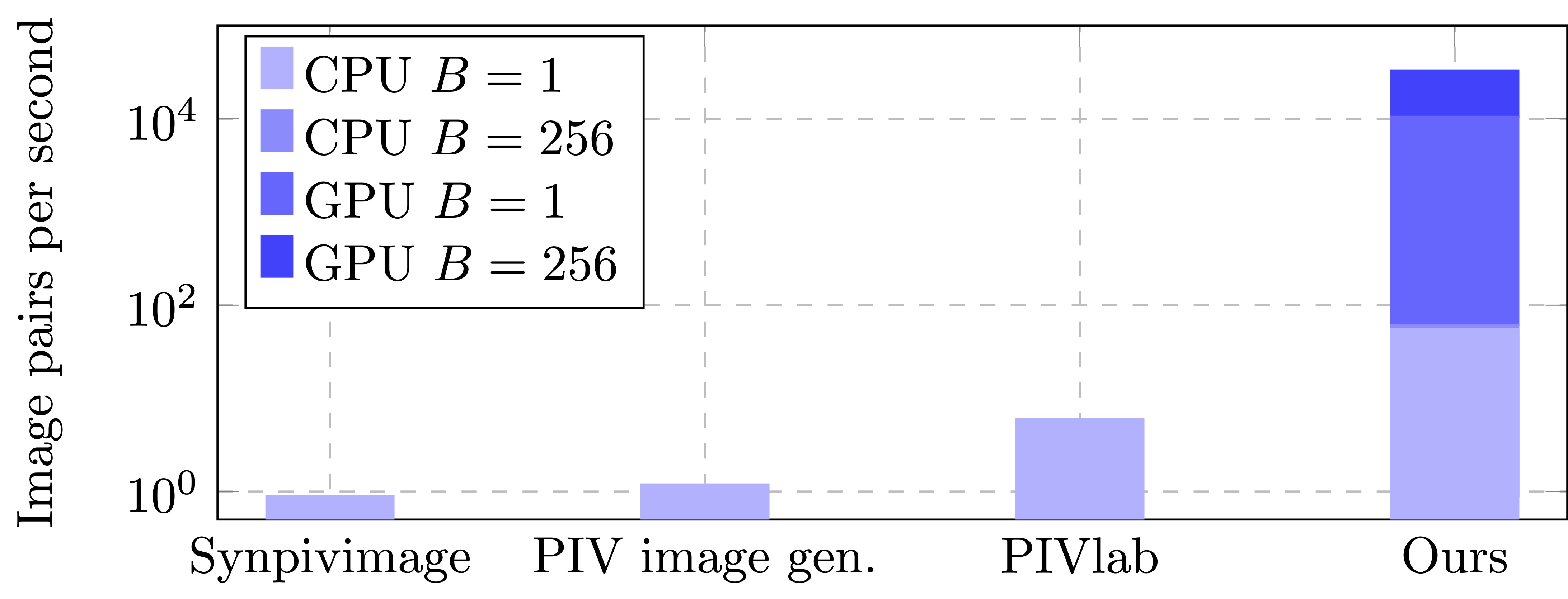
In a nutshell, if you need many synthetic PIV images and you do not want to wait ages, you are better off with SynthPix 😄. Below are the performances (image pairs per second) with and without GPU for different batch sizes B.

SynthPix is also fairly easy to use:

import synthpix

sampler = synthpix.make(config_path)
for i, batch in enumerate(sampler):
   """batch contains images1, images2, flow_fields, params"""
sampler.shutdown()

See src/main.py for a fully working example. For long-running training, check out our Checkpointing Guide to ensure bit-perfect reproducibility 💾.

Getting started 🚀

Alright, now that hopefully we convinced you to try SynthPix, let's get to it. Don't worry, installing it is even easier than using it:

uv add synthpix

If you have CUDA GPUs,

uv add "synthpix[cuda12]"

If you have issues with CUDA drivers, please follow the official instructions for cuda12 and cudnn (Note: wheels only available on linux). Make sure that LD_LIBRARY_PATH is not set; see the JAX docs:

unset LD_LIBRARY_PATH

Check out our instructions for installing SynthPix from source. You can of course also use pip.

To generate the images, you need flow data. We provide two scripts to download the commonly used PIV datasets:

sh scripts/download_piv_1.sh <output_folder> <configs_directory>

sh scripts/download_piv_2.sh <output_folder> <configs_directory>

These scripts will automatically save also one configuration file each in <configs_directory>. You can use these paths as in the example above.

For more examples and tutorials to use custom flow data or real-world data, check out our tutorials page.

Configuring the synthetic images ⚙️

Configuration is handled through a YAML file, organized into four main groups. Here’s a quick guide to what each set of parameters does:

1. Dataset Parameters

These parameters allow you to customize how flow field extraction works and the shape of the output batch.

Parameter	Description
seed	Random seed for reproducibility
batch_size	Number of image pairs generated at once
flow_fields_per_batch	Number of unique flow fields per batch
batches_per_flow_batch	Number of batches generated before updating to a new set of flow fields

2. Image Generation Parameters

Define the look and realism of your synthetic PIV images.

Parameter	Description
image_shape	Output image size [height, width] (pixels)
dt	Time between frames (seconds)
seeding_density_range	Range of particle densities (particles per pixel)
diameter_ranges	List of possible ranges for particle sizes (in pixels). (see below)
diameter_var	Variability in particle size
intensity_ranges	List of possible intensity (brightness) ranges. (see below)
intensity_var	Variability in intensity
p_hide_img1 / p_hide_img2	Per-particle probability of being hidden in image 1 (or 2).
rho_ranges	List of possible correlation coefficients ranges. (see below)
rho_var	Variability in correlation
noise_uniform	Maximum amplitude of uniform noise added to the image.
noise_gaussian_mean	Mean of Gaussian noise added to the image.
noise_gaussian_std	Standard deviation of Gaussian noise added to the image.
mask (optional)	Path to a .npy file containing a binary mask (0 and 1) with shape image_shape.
histogram (optional)	Path to a .npy file with a 1D array of shape (256,), summing to the number of image pixels. Used to remap output intensities.

For diameter_ranges, intensity_ranges, and rho_ranges, each parameter is a list of possible ranges. For every image pair, one range is randomly selected (uniformly) from each list, and then the particle parameters are sampled from these selected ranges.

Each *_var parameter controls how much the property of each particle can change between the first and second image of a pair. The change is applied as Gaussian noise with zero mean and variance given by the corresponding *_var value.

Here’s what each *_var parameter controls:

diameter_var: Simulates changes in particle size between frames, making the effect of focus, depth movement, or slight deformations more realistic.

Effect of diameter_var on particle size

Low Medium High

diameter = 2.0 diameter = 2.5 diameter = 3.0

_{Increasing diameter_var makes particles appear larger and more diffuse.}

intensity_var: Models natural brightness changes due to variations in illumination, camera response, or particles moving in and out of the light sheet mimicking out-of-plane motion.

Effect of intensity_var on particle brightness

Low Medium High

intensity = 50 intensity = 150 intensity = 255

_{Raising the intensity_var parameter produces brighter particles (higher signal-to-noise).}

rho_var: Adds variability to the shape and orientation (elongation/rotation) of particles between frames.

Effect of rho_var on particle shape:

Too Low Negative Zero Positive Too High

ρ = -0.9 ρ = -0.5 ρ = 0.0 ρ = 0.5 ρ = 0.9

_{Increasing the absolute value of rho (correlation coefficient) makes particle spots more elliptical and/or rotated.
Very high values (|ρ| > 0.5, leftmost and rightmost) lead to elongated, line-like particles that are not realistic for PIV images.
For best results, keep rho in the range -0.5 ≤ ρ ≤ 0.5.}

Note: The example above uses particles with diameter 2.5. The visual effect of ρ also depends on particle size, larger diameters make elongation more noticeable. As a result, the recommended "safe range" for realistic particle shapes may vary depending on your chosen diameter_ranges.

3. Flow generation parameters

Parameter	Description
velocities_per_pixel	Spatial resolution of the velocity field
resolution	Pixels per unit of physical length

Examples:

Use Case	velocities_per_pixel	resolution	Explanation
Normalized flow field	1.0	100	Flow field has 1 velocity vector per pixel; 100 px = 1 unit of length and flow velocity vectors are in units/s.
Real-world flow in m/s	10.0	50	Flow field has 10 velocity vectors per image pixel (very fine spatial resolution); 50 px = 1 meter and flow in m/s.
Pixel displacement flow	1.0	1.0	Flow field has 1 velocity per pixel; 1 px = 1 unit → flow directly describes pixels/second displacements. (use dt = 1 to convert it in pixels/frame)

4. Flow field parameters

Describe which region of your flow field is captured, and its velocity bounds.

Parameter	Description
flow_field_size	Physical size of the entire flow field (e.g., in mm × mm). Units must match those in your flow files.
img_offset	2D offset (in physical units, matching flow_field_size) specifying the top-left corner of the region of interest to extract from the flow field.
min_speed_x/y, max_speed_x/y	Range of allowed velocities in each direction,
output_units	Units used in the returned flow field: "pixels" (converts physical velocities to displacements in pixels using dt and resolution), or "measure units per second" (same units as the input flow field, e.g., mm/s).
file_list	List of ground-truth flow field files (e.g. .mat)
scheduler_class	Loader class for your flow files (usually by extension). See tutorials for detailed explanations.

Note: min_speed_x/y and max_speed_x/y are not absolute cutoffs, but define the full expected velocity range (positive and negative) along each axis.

These bounds are used to estimate the maximum particle displacement over time (dt). A larger intermediate image is generated accordingly, and the final image pair is cropped from this larger region. This ensures that particles entering the visible frame (image 2) have realistic origins — possibly outside the region of interest in image 1 — making particle "appearance" at the boundaries realistic.

Contributing 🤗

Contributions are more than welcome! 🙏 Please check out our how to contribute page, and feel free to open an issue for problems and feature requests⚠️.

Citation 📈

If you use this code in your research, please cite our paper:

   @misc{terpin2025synthpixlightspeedpivimages,
        title={SynthPix: A lightspeed PIV images generator},
        author={Antonio Terpin and Alan Bonomi and Francesco Banelli and Raffaello D'Andrea},
        year={2025},
        eprint={2512.09664},
        archivePrefix={arXiv},
        primaryClass={cs.DC},
        url={https://arxiv.org/abs/2512.09664},
    }